Stormwater Network (pipe network training)

Stormwater Network Design and Analysis in Devotech iDAS

For details about stormwater network design and analysis, watch the training videos

(login is required, sign up is for free, we need to approve your account, use company email address, if you need to use private email address, let us know on support@devotechgroup.com, we will approve it).

Open Devotech websites: https://www.devotechgroup.com/ and go to Education – Training Videos:

Sign in and go to the video channel Stormwater:

You can also find some useful tips in the Pipe Networks (General) video channel:

https://www.devotechgroup.com/pipe-networks-training

Catchments ─ Notes for Rational Method

Time of concentration (Tc) [1]

Devotech iDAS offers two Time of Concentration methods, the Kirpich and Kerby formulae.

Kirpich formula:

where: Tc = Time of Concentration (min),

L = Flow Length (m),

S = Slope (m/m).

Kerby formula:

where: Tc = Time of Concentration (min),

r = Retardance Roughness Coefficient,

L = Hydraulic Length of the Catchment (m),

S = Slope of the Catchment (m/m).

Typical values for the retardance roughness coefficient are shown in the table below:

Surface slope

If the Kirpich formula is used, the surface slope is calculated according to the rule 10-85:

If the Kerby formula is used, then the surface slope is calculated from the flow path start and end point elevation.

Minimum allowed Tc

Defines the minimum time of concentration, if the calculated Tc is shorter than the minimum allowed Tc, the minimum value is used.

Ascending limb multiplier

This value stretches (or shortens) the ascending limb of the computed triangular hydrograph when using the Rational hydrology method. The ascending limb of the runoff hydrograph occurs over the time duration obtained by multiplying this multiplier by the computed time of concentration (Tc). Therefore, the ascending limb is equal to Tc x Ascending Limb Multiplier. For example, if the Ascending Limb Multiplier is specified as 0.8, then the ascending side of the hydrograph would be 0.8 x Tc.

The image below shows a Limb Multiplier equal to 2.

Receding limb multiplier

This value stretches (or shortens) the receding limb of the computed triangular hydrograph when using the Rational hydrology method. The receding limb of the runoff hydrograph occurs over the time duration obtained by multiplying this multiplier by the computed time of concentration (Tc). Therefore, the receding limb is equal to Tc x Receding Limb Multiplier. For example, if the Receding Limb Multiplier is specified as 1.4, then the receding side of the hydrograph would be 1.4 x Tc. The image below shows a Limb Multiplier equal to 2.

Storm duration

The custom storm duration (SD) used for the analysis. If a custom storm duration should not be used, set the value to 0.

IDF Curves

The available IDF curves are from "The Civil Engineer in South Africa – March 1979" [2], see details on the next two pages. Users can also define a custom IDF curve in the Pipe Manager – tab Library – sub-tab IDF Curves.

Catchments ─ Notes for EPA SWMM Method

Average catchment slope

The catchment slope can be typed in or it can be calculated based on the Start-End rule from the reference surface

Equivalent width

Equivalent Width = Area / Flow Length

If the flow length is longer than 150m then:

Equivalent Width = Area / 150 (by the time the runoff has travelled circa 150m it has consolidated into rivulets and therefore no longer behaves as overland flow over a uniform plane).

Rain gage

Rain Gage is a rainfall distribution multiplied by a rainfall depth. Unit Rainfall available in the Devotech iDAS library represents the rainfall distribution.

South African rainfall distributions

The South African rainfalls distributions available in Devotech iDAS:

Regionalisation of rainfall temporal distribution in South Africa [3]:

The South African rainfall distribution graphs [3]:

Rainfall Depth for South African Regions

To obtain the rainfall depth for a specific weather station in South Africa, you can use the Design Rainfall software which can be downloaded from the following website:

https://ukzn-iis-02.ukzn.ac.za/unp/beeh/hydrorisk/RLMA%20and%20SI%20design%20rainfall.htm

To install and run the software, follow these steps:

Step 1:

Download the software (all three files):

Step 2:

Move all the files into one folder and unzip sagrid.zip file.

Step 3:

Copy SAgrid.dbf file from sagrid folder to the main folder:

Step 4

Since the Design Rainfall software is written in Java, you must install Java runtime environment by double clicking on j2re-1_4_0-win-i.exe:

Step 5

If you double click on rainfall3.jar file, the software should start up but on the latest Win 10 and Win 11 installation, double click just opens the rainfall3.jar folder.

The other option is to start up the application by using command Open With… from the right click menu. However, this option causes the application to not to provide any results or only the limited results:

To overcome this issue, the application must be started from the windows command line. Since many users are not familiar with the windows command line, it is easier to create a BAT file that will start up the application. Create a new Text Document in the same folder where all other files are saved by right clicking in the empty area and using command New – Text Document:

Created text file:

Open text file and insert the following text:

"C:\Program Files (x86)\Java\j2re1.4.0\bin\java.exe" -jar rainfall3.jar

Save the changes, close the text file, change the text file name to any suitable name and change the extension to .bat:

To start up the application**, double click on .bat file**. Specify the search method, duration, return period, location and click on Proceed. Save results to a file and open results in notepad.

Note: The Design Rainfall program implements procedures to estimate the design rainfall in South Africa developed by JC Smithers and RE Schulze. Funding for this project was obtained from the Water Research Commission through a project entitled "Rainfall Statistics for Design Flood Estimation in South Africa" (WRC Project K5/1060), and from the University of Natal Research Fund. Details of the procedures are contained in the WRC Report No. XXX/Y/2002 titled "Design Rainfall and Flood Estimation in South Africa" by JC Smithers and RE Schulze. The software was developed by MJ Gorven.

Any queries can be referred to:

School of Bio Resources Engineering and Environmental Hydrology

University of Natal

Private Bag X01

Scottsville

3201

South Africa

Telephone:033-2605490

Fax: 033-2605818

E-Mail: smithers@nu.ac.za

Import rainfall distribution and define rainfall depth

The rainfall distribution (Unit Rainfall) imported into the Pipe Manager Library under Unit Rainfalls:

To set the rainfall depth**,** go to ribbon Catchments and specify the values for each return period:

To assign Unit Rainfall to the catchments, select the catchments, right click and use command Unit Rainfall:

Impervious area (%)

The percentage of the catchment area that is impervious (i.e., roofs, asphalt or concrete roadways and sidewalks, etc.).

Impervious manning's roughness

Specify the Manning's roughness coefficient for overland flow over the impervious portion of the subbasin. The Manning's roughness value for overland flow is an effective roughness coefficient that includes the effect of raindrop impact; drag over the plane surface; obstacles such as litter, crop

ridges, and rocks; and erosion and transportation of sediment. Typical values are shown in the table below [4].

Pervious manning's roughness

Specify the Manning's roughness coefficient for overland flow over the pervious portion of the subbasin (i.e., grassy or open soil, etc.). The Manning's roughness value for overland flow is an effective roughness coefficient that includes the effect of raindrop impact; drag over the plane surface; obstacles such as litter, crop ridges, and rocks; and erosion and transportation of sediment. Typical values are shown in the table above.

Depression store impervious

Specify the depth of the depression storage on the impervious portion of the subbasin (mm). The surface storage is represented by a surface depression depth, such as localised depressions and other areas that will trap stormwater runoff, which must be satisfied before the runoff from impervious surfaces can begin. Note that this value is meant to account for "localised ponding" after a rainstorm, when little puddles are scattered around. Typical values are shown in the table below [4].

Depression store pervious

Specify the depth of the depression storage on the pervious portion of the subbasin (mm). The surface storage is represented by a surface depression depth, such as localised depressions and other areas that will trap stormwater runoff, which must be satisfied before runoff from impervious surfaces can begin. Generally, the surface storage (and the equivalent depression depth) is greater for pervious areas than impervious areas, as represented by a higher degree of surface irregularity.

Note that this value is meant to account for "localised ponding" that one will see after a rainstorm, when little puddles are scattered around.

Zero impervious (%)

Specify the percentage of the impervious area that has no depression storage, e.g. roofs.

Routing

Choice of the internal routing of runoff between pervious and impervious areas:

IMPERV:	runoff from pervious area flows to impervious area
PERV:	runoff from impervious flows to pervious area
OUTLET:	runoff from both areas flows directly to outlet

Routed

Percent of runoff routed between subareas.

Infiltration methods

Infiltration properties can be set in the Catchment Properties. Select any catchment and click on the Catchment Properties button (this command can also be accessed from the right-click menu).

Horton Infiltration

This infiltration method is based on empirical observations showing that infiltration decreases exponentially from an initial maximum rate to some minimum rate over the course of a long rainfall event. The input parameters required by this method include the maximum and minimum infiltration rates, a decay coefficient that describes how fast the rate decreases over time, and the time it takes fully saturated soil to completely dry. Max. Volume specifies the maximum possible infiltration volume in millimetres. If set to 0, then this field is not applicable.

The key advantages and limitations of the Horton infiltration method include:

• The Horton infiltration method is most likely to be important in urban and agricultural areas where the infiltration capacity of the soil is relatively small due to cultural activities.
• Because overland flow rarely occurs in forested soils, the Horton infiltration method is not applicable to these areas.

Typical infiltration rates [4]:

Catchments ─ Notes for Storm and Sanitary Analysis (SSA)

Import or create catchments in SSA

The catchments can either be created directly in SSA or imported from Civil 3D. If the catchments are in the same drawing as the pipe network, they will be exported along with the network, see chapter Export Network and Catchments from Civil 3D to SSA. For catchments in a separate drawing, refer to the Export Catchments to SSA chapter.

Catchments properties in SSA

To modify the catchment properties in SSA, double-click on the catchment centroid (the black rectangle in the middle of a catchment) to open a window where you can define the catchment properties. The available properties will vary depending to the settings under the Project Options. The Rational and EPA SWMM methods for runoff calculations use different catchment properties. The selected infiltration method (Horton, Green Ampt or SCS Curve) also influence the available catchment properties.

Project Options window:

Catchment Properties for Rational Method

The following physical properties must be specified: Area, Flow length and Average slope (10-85 rule or any other rule). The time of concentration is either calculated automatically according to the defined formula under the Project Options or it can be calculated manually.

Catchment Properties for EPA SWMM Method

The EPA SWMM method requires more physical properties to be specified, see the image below. The time of concentration is calculated automatically.

Equivalent Width = Area / Flow Length

If flow length is longer than 150m then:

Equivalent Width = Area / 150 (by the time runoff has travelled circa 150m it has consolidated into rivulets and therefore no longer behaves as overland flow over a uniform plane).

Infiltration Methods (only available when EPA SWMM method is selected)

SCS Curve Number Infiltration (default method)

This infiltration method is adapted from the NRCS (SCS) Curve Number method for estimating runoff. It assumes that the total infiltration capacity of the soil can be found from the soil's tabulated Curve Number. During a rain event this capacity is depleted as a function of cumulative rainfall and remaining capacity. The input parameters for this method are the curve number, the soil's hydraulic conductivity (used to estimate a minimum separation time for distinct rain events), and the time it takes fully saturated soil to completely dry.

The key advantages and limitations of the Curve Number infiltration method include:

• The Curve Number infiltration method continues to be most satisfactory when used for the type of hydrologic problem that it was developed to solve—evaluating effects of land use changes and conservation practices on direct runoff.
• The Curve Number infiltration method is less accurate when the runoff is less than 0.5 inches.
• When the weighted curve number is less than 40, use another infiltration method to determine the runoff.
• The Curve Number infiltration method is well established and widely accepted for use in the USA and abroad.
• It can be used for forested areas.
• The infiltration rate will approach zero during a storm of long duration, rather than a constant rate as expected.
• The default initial abstraction (0.2S) does not depend upon storm characteristics or timing.
• The rainfall intensity is not considered - same infiltration loss for 1 inch of rainfall in 1 hour or 1 day.
• The runoff from snow melt or rain on frozen ground cannot be estimated using the Curve Number infiltration method.

Horton Infiltration

This infiltration method is based on empirical observations showing that the infiltration decreases exponentially from an initial maximum rate to some minimum rate over the course of a long rainfall event. The input parameters required by this method include the maximum and minimum infiltration rates, a decay coefficient that describes how fast the rate decreases over time, and the time it takes fully saturated soil to completely dry.

The key advantages and limitations of the Horton infiltration method include:

• The Horton infiltration method is most likely to be important in urban and agricultural areas where the infiltration capacity of the soil is relatively small due to cultural activities.
• Because overland flow rarely occurs in forested soil, the Horton infiltration method is not applicable to these areas.

Green-Ampt Infiltration

This infiltration method assumes that a sharp wetting front exists in the soil column, separating the soil below with some initial moisture content from the saturated soil above. The input parameters required are the initial moisture deficit of the soil, the soil's hydraulic conductivity, and the suction head at the wetting front.

The key advantages and limitations of the Green-Ampt infiltration method include:

• The parameters of the Green-Ampt infiltration method can be related to soil properties that can be measured in a laboratory, such as porosity and hydraulic conductivity.
• The Green-Ampt infiltration method assumes an overland flow type mechanism which is not entirely appropriate for forested areas where a subsurface mechanism tends to control direct runoff.

Export Catchments to SSA

To export ONLY the catchments to SSA use the Devotech iDAS Parcels – Export Parcels command:

To import the catchments into SSA, use the same method used for a pipe network.

Time Steps

Four time steps must be specified: the runoff time steps for both wet weather and dry weather, a flow routing time step and a reporting time step. The most common error new users make is to use time steps that are too long. The Runoff Wet Weather time step should not exceed the precipitation recording interval. The flow Routing time step should never be larger than the wet weather time step, and in most cases should be 1 to 5 minutes (or less) for the Kinematic Wave routing and 30s (or less) for the Dynamic Wave routing. The Dynamic Wave routing can also employ a Variable Time Step option that automatically lowers the time step during periods when flows change rapidly. High continuity errors typically result when the runoff or routing time steps are too large. If the reporting time step is set too high, important details in the output results might be missed. Setting the reporting time step equal to the routing time step will prevent this but can generate very large output files.

Dynamic Wave Settings

The details about these settings can be found in the EPA SWMM help file.

Losses

Minor losses are only computed for the Dynamic Wave flow routing option. They are computed as Kv2/2g where K = minor loss coefficient, v = velocity, and g = acceleration of gravity. Entrance losses are based on the velocity at the entrance of the conduit, exit losses on the exit velocity, and average losses on the average velocity. The K value is influenced by many parameters and engineering judgment should be used when the K value is determined. Only enter data for conduits that have minor losses or flap valves.

ENTRY LOSS COEFFICIENT

The head loss coefficient associated with energy losses at the entrance of the conduit. For culverts, see the table in the EPA SWMM manual.

EXIT LOSS COEFFICIENT

The head loss coefficient associated with energy losses at the exit of the conduit. For culverts, use a value of 1.0. As a basic guide use the table below [4]:

Entry and Exit Loss Coefficients are properties of conduits within the SWMM engine, used for analyzing stormwater networks. However, in the Pipe Manager, these coefficients are located under Structures ─ Nodes:

During analysis, the values from structures are assigned to the corresponding conduits based on the following rules:

1. If the structure is at the start of a conduit, the structure Exit Loss Coefficient is used for the conduit Entrance Loss coefficient.
2. If the structure is at the end of a conduit, the structure Entrance Loss Coefficient is used for the conduit Exit Loss coefficient.

AVERAGE LOSS COEFFICIENT

Head loss coefficient associated with energy losses along the length of the conduit. It can be defined under Conduits – Pipes:

Manning’s Roughness Coefficient

Specify the conduit roughness coefficient in the Conduits tab**.** This coefficient is the Chezy-Manning roughness coefficient. The value can be set individually for each pipe, or for selected pipes, or for all pipes (right-click on the Friction Coeff column heading):

The typical values for Manning's roughness coefficients [4]:

Analysis Report

The analysis report can be viewed by clicking on the Analysis Report tab. It provides a summary of key results from the analysis.

Analysis Options

It displays the analysis settings that were applied during the analysis:

Flow routing continuity

You can check if the amount of water flowing into the system has the same volume as the water that is leaving the system. If these two volumes are not the same, you can check some settings:

1. Allow ponding setting allows overflow water to accumulate on top of the inlet structures. Once the system has capacity to handle the water again, it flows back into the system. If this option is enabled, it is crucial to define the ponding area for the inlet structures. Without this setting, any overflow water will be lost from the system.

2. Analysis duration might not be sufficient to empty the entire network. In this case, extend the analysis duration.

3. Storage nodes that have a specific volume for the irrigation. This volume never leaves the system.

In the example below, the inflow and outflow are equal and there are no flooding losses:

The other example below shows the discrepancy between inflow and outflow including the flooding loss. It also provides Final Stored Volume:

The Continuity Error indicates how well inflows and outflows balance. A lower error percentage suggests a more accurate simulation, confirming that inflows and outflows have been correctly modeled and accounted for.

Highest continuity errors

Some pipes or structures can show high continuity error:

This issue can arise from a variety of factors:

Hydraulic Modeling Limitations

If there are abrupt changes in flow direction or velocity, the model may struggle to maintain mass balance, resulting in high continuity errors.

Model Configuration Issues

Improper configuration of nodes and links can contribute to continuity errors. This includes misalignment of pipes, incorrect node elevations, or inappropriate boundary conditions that do not reflect real-world scenarios. Such misconfigurations can disrupt the expected flow paths and create inconsistencies in water balance.

Time Step Selection

The choice of time step for simulations can also impact continuity. A time step that is too large may not capture rapid changes in flow dynamics, while one that is too small may introduce numerical instability. Finding an appropriate balance is essential for accurate modeling.

Complex Flow Regimes

In urban environments, flow regimes can be complex due to interactions between surface runoff and drainage systems. Situations such as backwater effects or surcharging conditions can complicate the hydraulic calculations and lead to continuity errors if not adequately modeled

Pipe flow

The software computes the design flow capacity of a pipe for gravity flow conditions at 100% full (i.e., full flow conditions). The actual pipe capacity is higher (at about 94%).

Max/Full Depth should be below 0.8 (the pipe should not be more than 80% full, but various standards have different requirements).

Max/Full Flow should be below 1. If it is equal to 1 it means that there is pressure in the system which increases the flow in the pipe above the maximum pipe flow or the flow depth is close to the depth at which the maximum flow occurs, about 0.95% full.

Conditions which can occur [4]:

>CAPACITY

This condition is for example, reported when hydrodynamic routing is used and when the inflow is higher than the pipe capacity. A manhole is filling up with water and that creates pressure. A pipe can handle higher flow under pressure, but the flow depth is not constant in the pipe.

The longitudinal section with water surface (the image below is from Autodesk SSA software):

This behavior is very similar to culvert behavior where the capacity is driven either by the inlet or outlet structure [5]:

The link flow summary example for this scenario:

SURCHARGED

This condition is for example, reported when steady flow routing is used and if the inflow is higher than the pipe capacity. A manhole is filling up with water and that creates pressure. The Manning formula that is used for the steady flow analysis cannot handle flow under pressure.

Longsection with water surface:

The link flow summary example for this scenario:

CALCULATED but the results do not make sense

In some instances, the software reports that the Ratio of Maximum/Design Flow is equal to 1 and the Ratio of Maximum Flow Depth is 0.82, see the link flow summary below:

The longsection will not show any surcharging:

The software calculates the pipe capacity at 1D (100 % flow) and this capacity is very close to 0.8D (80% flow). Therefore, the capacity is fully used but the flow depth is close to 0.8.

Analysis Errors

Devotech iDAS uses the EPA SWMM engine for analysis. Below is a list of possible errors which can occur during the analysis. This list was copied from the EPA SWMM User's Manual [6].

ERROR 101: memory allocation error.

There is not enough physical memory in the computer to analyse the study area.

ERROR 103: cannot solve KW equations for Link xxx.

The internal solver for the Kinematic Wave routing failed to converge for the specified link at some stage of the simulation.

ERROR 105: cannot open ODE solver.

The system could not open its Ordinary Differential Equation solver.

ERROR 107: cannot compute a valid time step.

A valid time step for the runoff or flow routing calculations (i.e., a number greater than 0) could not be computed at some stage of the simulation.

ERROR 108: ambiguous outlet ID name for Subcatchment xxx.

The name of the element identified as the outlet of a subcatchment belongs to both a node and a subcatchment in the project's data base.

ERROR 109: invalid parameter values for Aquifer xxx.

The properties entered for an aquifer object were either invalid numbers or were inconsistent with one another (e.g., the soil field capacity was higher than the porosity).

ERROR 111: invalid length for Conduit xxx.

Conduits cannot have zero or negative lengths.

ERROR 112: elevation drop exceeds length for Conduit xxx.

The elevation drop across the ends of a conduit cannot be greater than the conduit's length. Check for errors in the length and in both the invert elevations and offsets at the conduit's upstream and downstream nodes.

ERROR 113: invalid roughness for Conduit xxx.

Conduits cannot have zero or negative roughness values.

ERROR 114: invalid number of barrels for Conduit xxx.

Conduits must consist of one or more barrels.

ERROR 115: adverse slope for Conduit xxx.

Under Steady or Kinematic Wave routing, all conduits must have positive slopes. This can usually be corrected by reversing the inlet and outlet nodes of the conduit (i.e., right-click on the conduit and select Reverse from the popup menu that appears). Adverse slopes are permitted under Dynamic Wave routing.

ERROR 117: no cross section defined for Link xxx.

Cross-section geometry was never defined for the specified link.

ERROR 119: invalid cross section for Link xxx.

Either an invalid shape or invalid set of dimensions was specified for a link's cross-section.

ERROR 121: missing or invalid pump curve assigned to Pump xxx.

Either no pump curve or an invalid type of curve was specified for a pump.

ERROR 131: the following links form cyclic loops in the drainage system.

The Steady and Kinematic Wave flow routing methods cannot be applied to systems where a cyclic loop exists (i.e., a directed path along a set of links that begins and ends at the same node). Most often the cyclic nature of the loop can be eliminated by reversing the direction of one of its links (i.e., switching the inlet and outlet nodes of the link). The names of the links that form the loop will be listed following this message.

ERROR 133: Node xxx has more than one outlet link.

Under Steady and Kinematic Wave flow routing, a junction node can only have a single outlet link.

ERROR 134: Node xxx has more than one DUMMY outlet link.

Only a single conduit with a DUMMY cross-section can be directed out of a node.

ERROR 135: Divider xxx does not have two outlet links.

The flow divider nodes must have two outlet links connected to them.

ERROR 136: Divider xxx has invalid diversion link.

The link specified as being the one carrying the diverted flow from a flow divider node was defined with a different inlet node.

ERROR 137: Weir Divider xxx has invalid parameters.

The parameters of a Weir-type divider node either have non-positive numbers or are inconsistent (i.e., the value of the discharge coefficient times the weir height raised to the 3/2 power must be greater than the minimum flow parameter).

ERROR 138: Node xxx has initial depth greater than maximum depth.

Self-explanatory.

ERROR 139: Regulator xxx is the outlet of a non-storage node.

Under Steady or Kinematic Wave flow routing, orifices, weirs, and outlet links can only be used as outflow links from storage nodes.

ERROR 141: Outfall xxx has more than 1 inlet link or an outlet link.

An outfall node is only permitted to have one link attached to it.

ERROR 143: Regulator xxx has invalid cross-section shape.

An orifice must have either a CIRCULAR or RECT_CLOSED shape, while a weir must have either a RECT_OPEN, TRAPEZOIDAL, or TRIANGULAR shape.

ERROR 145: Drainage system has no acceptable outlet nodes.

Under the Dynamic Wave flow routing, there must be at least one node designated as an outfall.

ERROR 151: a Unit Hydrograph in set xxx has invalid time base.

The time base of a Unit Hydrograph cannot be negative and if positive, must not be less than the recording interval for its rain gage.

ERROR 153: a Unit Hydrograph in set xxx has invalid response ratios.

The response ratios for a set of Unit Hydrographs (the short-, medium-, and long-term response hydrographs) must be between 0 and 1.0 and cannot add up to a value greater than 1.0

ERROR 155: invalid sewer area for RDII at Node xxx.

The sewer area contributing RDII inflow to a node cannot be a negative number.

ERROR 157: inconsistent rainfall format for Rain Gage xxx.

If two or more rain gages use the same Time Series for their rainfall data then they must all use the same data format (intensity, volume, or cumulative volume).

ERROR 159: inconsistent time interval for Rain Gage xxx.

The recording time interval specified for the rain gage is greater than the smallest time interval between values in the Time Series used by the gage.

ERROR 161: cyclic dependency in treatment functions at Node xxx.

An example would be where the removal of pollutant 1 is defined as a function of the removal of pollutant 2 while the removal of pollutant 2 is defined as a function of the removal of pollutant 1.

ERROR 171: Curve xxx has its data out of sequence.

The X-values of a curve object must be entered in increasing order.

ERROR 173: Time Series xxx has its data out of sequence.

The time (or date/time) values of a time series must be entered in sequential order.

ERROR 181: invalid Snow Melt Climatology parameters.

The ATI Weight or Negative Melt Ratio parameters are not between 0 and 1 or the site latitude is not between -60 and +60 degrees.

ERROR 182: invalid parameters for Snowpack xxx.

A snowpack's minimum melt coefficient is greater than its maximum coefficient; the fractions of free water capacity or impervious plowable area are not between 0 and 1; or the snow removal fractions sum to more than 1.0.

ERROR 191: simulation start date comes after ending date.

Self-explanatory.

ERROR 193: report start date comes after ending date.

Self-explanatory.

ERROR 195: reporting time step is less than routing time step.

Self-explanatory.

ERROR 200: one or more errors in input file.

This message appears when one or more input file parsing errors (the 200-series errors) occur.

ERROR 201: too many characters in input line.

A line in the input file cannot exceed 1024 characters.

ERROR 203: too few items at line n of input file.

Not enough data items were supplied on a line of the input file.

ERROR 205: invalid keyword at line n of input file.

An unrecognized keyword was encountered when parsing a line of the input file.

ERROR 207: duplicate ID name at line n of input file.

An ID name used for an object was already assigned to an object of the same category.

ERROR 209: undefined object xxx at line n of input file.

A reference was made to an object that was never defined. An example would be if node 123 were designated as the outlet point of a subcatchment, yet no such node was ever defined in the study area.

ERROR 211: invalid number xxx at line n of input file.

Either a non-numeric character was encountered where a numerical value was expected or an invalid number (e.g., a negative value) was supplied.

ERROR 213: invalid date/time xxx at line n of input file.

An invalid format for a date or time was encountered. Dates must be entered as month/day/year and times as either decimal hours or as hour:minute:second.

This error might appear although the setting is correct. Changing the time format should solve this issue.

1. Close Civil 3D

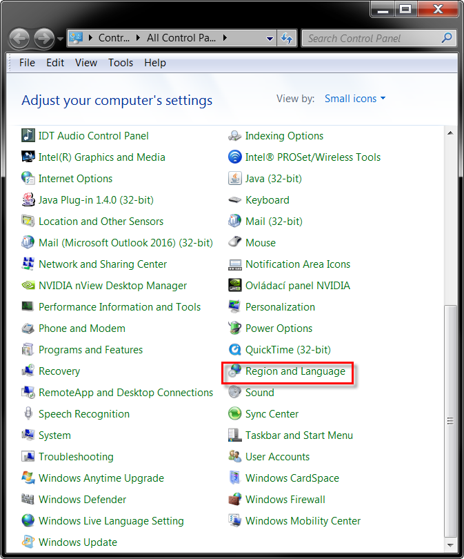
2. Open the Control Panel and click on Region and Language:

   

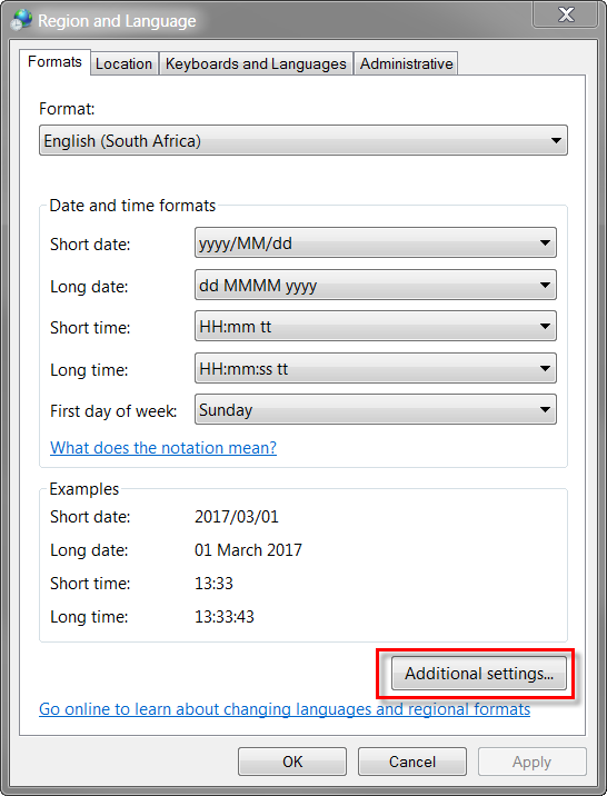
3. Click on Additional Settings:

   

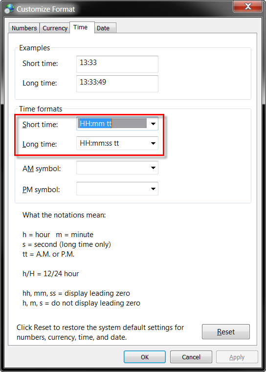
4. Set Short and Long times according to the image below:

   

ERROR 217: control rule clause out of sequence at line n of input file.

Errors of this nature can occur when the format for writing control rules is not followed correctly (see Section C.3).

ERROR 219: data provided for unidentified transect at line n of input file.

A GR line with Station-Elevation data was encountered in the [TRANSECTS] section of the input file after an NC line but before any X1 line that contains the transect's ID name.

ERROR 221: transect station out of sequence at line n of input file.

The station distances specified for the transect of an irregular cross-section must be in increasing numerical order starting from the left bank.

ERROR 223: Transect xxx has too few stations.

A transect for an irregular cross-section must have at least 2 stations defined for it.

ERROR 225: Transect xxx has too many stations.

A transect cannot have more than 1500 stations defined for it.

ERROR 227: Transect xxx has no Manning's N.

No Manning's N was specified for a transect (i.e., there was no NC line in the [TRANSECTS] section of the input file.

ERROR 229: Transect xxx has invalid overbank locations.

The distance values specified for either the left or right overbank locations of a transect do not match any of the distances listed for the transect's stations.

ERROR 231: Transect xxx has no depth.

All the stations for a transect were assigned the same elevation.

ERROR 233: invalid treatment function expression at line n of input file.

A treatment function supplied for a pollutant at a specific node is either not a correctly formed mathematical expression or refers to unknown pollutants, process variables, or math functions.

ERROR 301: files share same names.

The input, report, and binary output files specified on the command line cannot have the same names.

ERROR 303: cannot open input file.

The input file either does not exist or cannot be opened (e.g., it might be in use by another program).

ERROR 305: cannot open report file.

The report file cannot be opened.

Problem 1: A drawing might reside in a directory to which the user does not have write privileges.

Solution: Move the drawing to your desktop, open it from this new location and rerun the analysis.

Problem 2: Multiple Civil 3D instances are causing the issue.

Solution: Close all running Civil 3D instances for all the Civil 3D versions and start up only one Civil 3D instance.

Problem 3: Civil 3D limits the access to the location where the drawing is saved.

Solution: Set the folder where the drawing is saved as a trusted location. Open Civil 3D Options:

Select the Trusted Location folder, click on Add and browse to the folder where the drawing is saved. If you want to include the selected folder as well as its subfolders, you must add three dots "…" at the end of the folder path:

Problem 4: The drawing path or drawing name is too long.

Solution: Move the drawing to a folder with the shorter path or rename the drawing.

Problem 5: Civil 3D does not have a privilage to create file in the location where the drawing is saved.

Solution: Run Civil 3D as administrator (right click on the Civil 3D icon and use Run as administrator command)

Problem 6: The user's antivirus is blocking the temporary file which is created by Devotech iDAS in the location where the drawing is saved when running the analysis.

Solution: Create an exception rule on the firewall to allow access to EPA SWMM and SSA.

Problem 7: The user is using Bentley Project Wise and it does not allow the user to create that file type on the system.

Solution: Move the drawing to the C drive and then run the analysis.

ERROR 307: cannot open binary results file.

The binary output file cannot be opened (e.g., it might reside in a directory to which the user does not have write privileges).

ERROR 309: error writing to binary results file.

There was an error in trying to write results to the binary output file (e.g., the disk might be full, or the file size exceeds the limit imposed by the operating system).

ERROR 311: error reading from binary results file.

The command line version of SWMM could not read results saved to the binary output file when writing results to the report file.

ERROR 313: cannot open scratch rainfall interface file.

SWMM could not open the temporary file it uses to collate data together from external rainfall files.

ERROR 315: cannot open rainfall interface file xxx.

SWMM could not open the specified rainfall interface file, possibly because it does not exist or because the user does not have write privileges to its directory.

ERROR 317: cannot open rainfall data file xxx.

An external rainfall data file could not be opened, most likely because it does not exist.

ERROR 319: invalid format for rainfall interface file.

SWMM was trying to read data from a designated rainfall interface file with the wrong format (i.e., it may have been created for some other project or another type of file).

ERROR 321: no data in rainfall interface file for gage xxx.

This message occurs when a project wants to use a previously saved rainfall interface file, but it cannot find any data for one of its rain gages in the interface file.

ERROR 323: cannot open runoff interface file xxx.

A runoff interface file could not be opened, possibly because it does not exist or because the user does not have write privileges to its directory.

ERROR 325: incompatible data found in runoff interface file.

SWMM was trying to read data from a designated runoff interface file with the wrong format (i.e., it may have been created for some other project or another type of file).

ERROR 327: attempting to read beyond end of runoff interface file.

This error can occur when a previously saved runoff interface file is being used in a simulation with a longer duration than the one that created the interface file.

ERROR 329: error in reading from runoff interface file.

A format error was encountered while trying to read data from a previously saved runoff interface file.

ERROR 331: cannot open hotstart interface file xxx.

A hotstart interface file could not be opened, possibly because it does not exist or because the user does not have write privileges to its directory.

ERROR 333: incompatible data found in hotstart interface file.

SWMM was trying to read data from a designated hotstart interface file with the wrong format (i.e., it may have been created for some other project or another type of file).

ERROR 335: error in reading from hotstart interface file.

A format error was encountered while trying to read data from a previously saved hotstart interface file.

ERROR 336: no climate file specified for evaporation and/or wind speed.

This error occurs when the user specifies that evaporation or wind speed data will be read from an external climate file, but no name is supplied for the file.

ERROR 337: cannot open climate file xxx.

An external climate data file could not be opened, most likely because it does not exist.

ERROR 338: error in reading from climate file xxx.

SWMM was trying to read data from an external climate file with the wrong format.

ERROR 339: attempt to read beyond end of climate file xxx.

The specified external climate does not include data for the time period being simulated.

ERROR 341: cannot open scratch RDII interface file.

SWMM could not open the temporary file it uses to store RDII flow data.

ERROR 343: cannot open RDII interface file xxx.

An RDII interface file could not be opened, possibly because it does not exist or because the user does not have write privileges to its directory.

ERROR 345: invalid format for RDII interface file.

SWMM was trying to read data from a designated RDII interface file with the wrong format (i.e., it may have been created for some other project or another type of file).

ERROR 351: cannot open routing interface file xxx.

A routing interface file could not be opened, possibly because it does not exist or because the user does not have write privileges to its directory.

ERROR 353: invalid format for routing interface file xxx.

SWMM was trying to read data from a designated routing interface file with the wrong format (i.e., it may have been created for some other project or another type of file).

ERROR 355: mismatched names in routing interface file xxx.

The names of pollutants found in a designated routing interface file do not match the names used in the current project.

ERROR 357: inflows and outflows interface files have same name.

In cases where a run uses one routing interface file to provide inflows for a set of locations and another to save outflow results, the two files cannot both have the same name.

ERROR 361: could not open external file used for Time Series xxx.

The external file used to provide data for the named time series could not be opened, most likely because it does not exist.

ERROR 363: invalid data in external file used for used for Time Series xxx.

The external file used to provide data for the named time series has one or more lines with the wrong format.

Analysis Warnings

WARNING 01: wet weather time step reduced to recording interval for Rain Gage xxx.

The wet weather time step was automatically reduced so that no period with rainfall would be skipped during a simulation.

WARNING 02: maximum depth increased for Node xxx.

The maximum depth for the node was automatically increased to match the top of the highest connecting conduit.

WARNING 03: negative offset ignored for Link xxx.

The link's stipulated offset was below the connecting node's invert, its actual offset was set to 0.

WARNING 04: minimum elevation drop used for Conduit xxx.

The elevation drop between the end nodes of the conduit was below 0.001ft (0.00035m), the latter value was used instead to calculate its slope.

WARNING 05: minimum slope used for Conduit xxx.

The conduit's computed slope was below the user-specified Minimum Conduit Slope, the latter value was used instead.

WARNING 06: dry weather time step increased to wet weather time step.

The user-specified time step for computing runoff during dry weather periods was lower than that set for wet weather periods and was automatically increased to the wet weather value.

WARNING 07: routing time step reduced to wet weather time step.

The user-specified time step for flow routing was larger than the wet weather runoff time step and was automatically reduced to the runoff time step to prevent loss of accuracy.

Update Profile View and Part Properties

To write all the input values and analysis results to the pipes' and structures' properties tick the Update Results to C3D option Pipe Manager and click Update. As a default this option is ticked off because it takes longer to write all the values in the pipe and structure properties:

Values written to the structure properties:

Values from the analysis are automatically displayed in the profile view:

Surface Channels Analysis

What is surface channel

Surface channel is a channel that is formed by a surface. It can be a surveyed surface (NGL), or it can be a surface created from a corridor, for example road or channel.

Road as a channel:

NGL surface channel:

Create surface channel

In order to be able to add a surface channel to the Pipe Manager, the drawing must contain the following items:

1. Horizontal alignment with sample lines that must sample the source surface which forms the surface channel

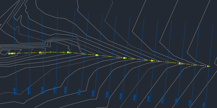   Sampled source surface (in this case NGL surface) under Sample Line Group properties: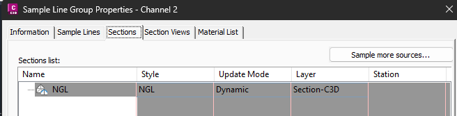

   

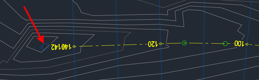
2. Pipe network with outfall structure that will be used as a surface channel outfall. The rim and sump outfall elevations are not important because surface channels connects to outfall with the direct link in the analytical model.

   

3. Orphan pipe with two structures. The reason for the orphan pipe with two structures is that the Pipe Manager does not load a network that does not contain at least one pipe. This pipe has no impact on the analysis. Any pipe type and structure type can be used for orphan pipe with structures. If you have a culvert along the channel, you do not need to create the orphan pipe because the culvert contains a pipe. Example of orphan pipe with two structures:

   

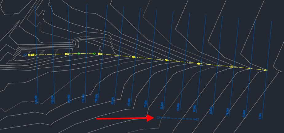
Open Pipe Manager and click on command Add Surface Channel in the Surface Channels tab:

Select horizontal alignment(s), hit enter and when the command returns back to Pipe Manager, the surface channel will be displayed in the list:

Specify Sample Line Group, Channel Surface, Flow to Node (this can be an outfall structure or node from a pipe network) and Manning Coefficient:

If you go to Sections tab and select any cross-section in the list, it will display the section location in plan and the actual cross-section:

The first section view is intentionally empty due to the way the model is constructed. Sample lines represent the structures, while the sections at those sample lines are used to define the geometry of the channel conduits.

The section at the second sample line is used to define the geometry of the upstream channel conduit. As a result, the first section is not associated with any conduit because there is no conduit upstream of the first structure.

Similarly, the section at the last sample line is used to define the geometry of the final channel conduit in the model.

The Sections list allows to specify the following properties:

• Direct Inflow – to specify direct inflow.
• Flow from Surface Channel - to introduce inflow from other channels and link them together. The analytical model uses Direct link to connect surface channels.
• Flow from Node – to introduce inflow from pipe network structures and link them together. The analytical model uses Direct link to connect structures with surface channels.
• Flow to Node and Overflow – it introduces the flow to the selected structure and if there is no capacity in the outgoing pipe, it overflows back to the surface channel. Since EPASWMM analytical engine does not support more than two direct links to be connected to a node (for flow in and out), the selected node is used as a surface channel node. For more details see the chapter related to using surface channels for overflows.
• Limit Flow – to limit the maximum flow through the channel. If set to 0, no limit is set.
• Manning's Roughness Coefficient – set the roughness coefficient for each section individually.
• Entrance Loss Coefficient and Exit Loss Coefficient – specify the entrance and exit losses for each channel conduit. It is important to note that, within the SWMM engine, these properties are properties of conduits, whereas a channel section is represented as a junction node (structure) within the SWMM engine. Because of this, during the analysis, the loss coefficients defined for sections are automatically assigned to the corresponding channel conduits according to the following rules:
  • If the section is located at the start of a channel conduit, the section's Exit Loss Coefficient is assigned as the conduit Entrance Loss Coefficient.
  • If the section is located at the end of the channel conduit, the section's Entrance Loss Coefficient is assigned as the conduit Exit Loss Coefficient.
• Average Loss Coefficients – specify the energy losses along the conduit. The section at the second sample line is used to define the geometry of the upstream channel conduit. As a result, define the Average Loss Coefficient for the first channel conduit under the second sections. The Average Loss Coefficient from the first section is not used because there is no conduit upstream of the first structure.

The Profile tab displays the profile view:

Navigation in profile view

Click on the sample line chainages to display specific cross-section:

Use sliders at the bottom of the profile view to zoom to a specific profile area:

Analyse surface channels

To analyse surface channels, use Analyse command as you would use for any other pipe network. Surface channels are part of the pipe network because they must always flow to a node (outfall or pipe network structure):

Preview analysis results

The results can be previewed in the Reports tab, Analysis Report subtab. Surface channel node names have prefix SCN#, where SCN means Surface Channel Node, and # means the surface channel number (it is assigned automatically) followed by underscore and sample line name:

Surface channel link names have prefix SCC#, where SCC means Surface Channel Conduit, and # means the surface channel number (it is assigned automatically) followed by underscore and sample line name:

Note: The surface channel nodes and links are not displayed under summary results:

The results can also be previewed in the Surface Channels tab, Section subtab:

And in the Surface Channels tab, Profiles subtab, which displays graphically the following results:

• Top conduit water elevation
• Top node water elevation
• EGL
• Lowest invert elevation (it does not need to be at the channel centerline)
• Maximum velocity
• Maximum flow
• Section location

Export results (profiles) to Civil 3D

The profiles from the Profiles tab can be exported to Civil 3D with the commands at the top of the Surface Channels tab (the profiles can also be updated with these commands):

The following profiles can be exported or updated:

• Max conduit water Profile
• Max node water Profile
• Max EGL profile
• Invert profile
• Max flow profile
• Max velocity profile
• Min freeboard profile

The last profile created or updated of each type will be listed in the Result Profiles column and will be automatically updated with every successful analysis. To remove a profile from the list of automatically updated profiles, click a profile button and select <None> as the profile name.

Use surface channels for overflows

Surface channels can be used for stormwater networks overflows. The water can flow from a road (surface channel) into a pipe network inlet. If the inlet does not have a capacity, it will overflow along the road to the next inlet and so on. The inlet structures can be treated as flow dividers, which allow to specify the inlet's capacity by using different divider types (Cutoff, Overflow, Tabular, Wier):

Important: If you use flow dividers, the Kinematic Wave or Steady Flow routing must be used otherwise the dividers are treated as normal junctions and divider types and settings are ignored:

Prepare object in Civil 3D model space

The image below shows the starting point with the road corridor, corridor top surface and pipe network with inlet structures, manholes, network outfall and channel outfall (all these objects belong to one network; pipe network is designed vertically):

Create sample lines at interval for the road alignment and sample corridor top surface:

Created sample lines:

Add additional sample lines at the pipe network inlet structures locations:

Additional sample lines:

Set up and analyse model in Pipe Manager

Open Pipe Manager, add surface channel and define the properties (as a Flow to Node use channel outfall):

If a surface channel node should flow to inlet structure then set the inlet structure as Flow to Node and Overflow in the Sections tab**:**

Pipe Manager will display dashed line with an arrow between the surface channel node and inlet structure to visually show the relationship:

Set the manning coefficient for each of the surface channel section. To fill in multiple sections at once the grid can be right-clicked on and the Manning Coefficient… option chosen.

Set the pipe network pipe's roughness coefficient:

Run the analysis:

Analytical model explanation

When an inlet structure is assigned for Flow to Node and Overflow, then the channel node is replaced with the inlet structure and the channel continues from the inlet structure to next channel flow. Since the distance from inlet structure to the next channel flow differs from the original distance, the original length is used for the link length.

There are two reasons for using this approach:

1. is that a node can only have one direct link connected and it is reserved for Flow from Node link. Direct link is a link that does not have any hydraulics and introduces the flow directly to a specified node.

Below is an example of Pipe Manager model on the lefthand side and the analytical model displayed in SSA on the righthand side. The surface channel nodes at positions 1, 4, and 6 were replaced with the inlet structures:

Surface channels with culverts

Surface channels can have other objects along the route, such as culverts. In this case, the culvert inlet structure behaves as an overflow structure and should be mapped as a divider with a very high Cutoff value (e.g.: 100 m3) to prevent any overflow back to the channel. The channel analytical model runs along the culvert but does not have any flow:

Prepare object in Civil 3D model space

The image below shows the alignment used to model the surface channel and pipe network with a culvert and structure headwalls (all these objects belong to one network; pipe network is designed vertically):

Create sample lines at interval for the channel alignment and sample the surface:

Created sample lines:

Add and or remove sample lines so that there are no sample lines crossing the culvert and that there is a sample line close to the start and end of the culvert:

Set up and analyse model in Pipe Manager

Open Pipe Manager, add surface channel and define the properties (as a Flow to Node use channel outfall):

For the sample line that is close to the inlet headwall set the Flow to Node and Overflow to the inlet headwall structure. For the sample line that is close to the outlet headwall set the Flow from Node to the inlet headwall structure. Fill in a manning coefficient for each channel section.

Pipe Manager will display dashed line with an arrow between the surface channel node and inlet and outlet headwall structures to visually show the relationship:

When a structure is assigned to a sample line's Flow to Node and Overflow property the default behavior is that if the structure cannot absorb all the flow then it will overflow back into the surface channel. When all the flow must go into the structure (as in the case of a culvert) the structure will need to be modelled as a Divider so that the flow can be cut off and forced into the culvert.

To achieve this swap the inlet headwall structure to a divider (or update the structure mappings and assign the inlet headwall structure as a divider). Then in the Dividers tab tick on the Divert to Surface Channel, change the Diversion Type to Cutoff and put a large value in the Cutoff Flow column. What this is doing is it is forcing and overflow back into the channel (instead of another connected pipe) and then is preventing the flow from being diverted into the channel until the flow exceeds the Cutoff Flow. That is why a large value is used, it should be a value larger than any possible flow through the channel. In this example 100m3 was supplied.

Analytical model explanation

When the culvert inlet headwall structure is assigned to Flow to Node and Overflow, then the surface channel node is replaced with the inlet structure and the channel continues from the inlet structure to next channel section. In this case we do not want the surface channel to run parallel to our culvert so a divider has to be used to prevent flow back into the surface channel.

Below is an example of Pipe Manager model on the lefthand side and the analytical model displayed in SSA on the righthand side. Note the parallel lines in the analytical model. The top line is the surface channel running next to the culvert and has its flow cut off, therefore it is essentially not used in the analysis.

Note that this type of modelling using a divider to cut off the flow does not work if the routing model is set to Dynamic Wave. If using dynamic wave then a divider is not needed and the junction should be kept. In order to restrict the flow from flowing in the surface channel instead of the culvert the Limit Flow column can be used. By default the Limit Flow value is set to zero, which means that the flow will not be limited. If a value is provided then the flow will be limited. To disable the flow, use a very small number (e.g. 0.000001 m3/s) for the section that is parallel to the culvert:

Dynamic Wave Notes

If a channel has adverse slopes then the Dynamic Wave method must be used because Steady Flow and Kinematic Wave methods do not support adverse slopes.

Dynamic Wave behaves differently from Steady Flow and Kinematic Wave methods. The following sections discuss some unexpected results when using Dynamic Wave, and what can be done to produce more accurate results where possible.

Conduit depths

When using the Dynamic Wave method, conduit flow depths are calculated from the flow depths of the connected nodes. If conduits are connected in parallel to the same upstream and downstream nodes, and the flow in the conduits differs, the flow depth will be reported as equal. This is because both conduits are connected to the same nodes, thus they will report the same depth.

With the Dynamic Wave method the flow depth can be different along the length of a conduit (as determined by the depth at the connected nodes). The Steady Flow and Kinematic Wave methods calculate the flow depth as being constant across the entire length of the conduit. Although the flow depth is different across the conduit when using the Dynamic Wave method, the EPA SWMM engine reports the flow depth of a conduit as a single value. This value is a sort of average calculated from the flow depths at the connected nodes.

The flow depth behavior described above can be seen in the surface channels when introducing a conduit in place of a section of the surface channel. In the image below a culvert has been introduced between stations 49.894m and 70.382m. As can be seen in the results table the design flow for the surface channel between those stations was limited to 0.000001m3/s resulting in a design flow of 0.000m3/s and a flow depth of 1.200m. In the graph the dark blue line is the flow depth of the surface channel conduits, and as can be seen from the image below, the flow depth is greater than zero even though the flow through the conduit section is zero. The graph also shows the difference between the flow depths at the nodes (light blue line) and the flow depth in the conduits (dark blue line).

In contrast, the image below shows the results of the same model which was analyzed with the Steady Flow method. As you can see the portion of the surface channel that was replaced with a conduit reports the flow depth as zero. This is because the Steady Flow and Kinematic Wave methods do not use the node flow depths to calculate the conduit flow depths but instead use the design flow to determine the depth with the assumption that the flow depth is constant in a conduit.

Incorrect flow depth at end of surface channel

When determining the flow depth at a node, the Dynamic Wave method uses the connected conduits' shape to determine the depth. When a "dummy" conduit is used the flow depth of the node will be much less than what is expected because a "dummy" conduit has no shape and just transfers the flow from one node to another. This causes the flow depth at the node connected to the "dummy" conduit to be very shallow, and in return it will cause the conduit's flow depth to also be less than expected.

"Dummy" conduits are used to connect the end of a surface channel to a structure, as well as connecting inflow structures and inflow surface channels.

In the image below the surface channel is connected to structure MH8 in the Flow to Node column. In the analytical model a "dummy" conduit is created between the end of the surface channel and structure MH8. This results in the flow depth at the final node of the surface channel being less than expected.

To prevent the flow depth from being reduced at the last node, the Flow to Node can be set to <None> and the Flow to Node and Overflow for the last section can be set to the outlet structure (MH8 in this example). This will prevent the "dummy" link from being created and will instead connect the surface channel directly to the structure as specified by the Flow to Node and Overflow column.

The image below is the result of the change above. The flow depth is now correct for the last section of the surface channel.

Incorrect flow depth when connecting to a free or normal outfall

When connecting a surface channel to an outfall that is of type free or normal, the flow depth of the final section of the surface channel may reduce to zero as seen in the image below.

This happens when the outfall invert level (structure sump elevation) is lower than the connected conduits invert level at the outfall. When using the Dynamic Wave method, EPA SWMM needs to calculate the critical and normal flow depths under certain circumstances as documented in the EPA Storm Water Management Model Reference Manual [7]:

5.5 Critical and Normal Depths

SWMM needs to calculate the critical and normal flow depths in a conduit for dynamic wave

analysis whenever:

1. the conduit is connected to a free outfall node

2. a discontinuity exists between the water level in the conduit and in its connecting node

(i.e. a free fall condition exists). These depths are functions of flow rate and cross section shape. For all but the simplest shapes, iterative numerical methods are required to compute them.

Since EPA SWMM only allows one conduit to be attached to an outfall, and there is a difference in elevation between the conduit and the outfall, the engine does not know if a free fall condition exists and defaults to a flow depth of zero at the outfall.

This can be remedied by ensuring the outfall level (structure sump elevation) is the same as the lowest invert elevation of the last surface channel section. Setting the outfall level correctly results in the water depth being calculated correctly as seen in the image below:

Pond Design Notes

We are preparing a video for Devotech iDAS 12 detention pond design. Below are the tables with the orifice and weir coefficients.

Orifice Discharge Coefficients

See the user table below for the orifice discharge coefficients. This table was copied from the Autodesk Storm and Sanitary analysis help file [4]:

Weir Discharge Coefficients

See the user table below for the orifice discharge coefficients. This table was copied from the Autodesk Storm and Sanitary analysis help file [4]:

Stormwater Network Analysis in SSA

The Devotech iDAS users can run the analysis in Devotech iDAS or in Autodesk SSA.

Note: Storm and Sanitary Analysis (SSA) software is part of the Civil 3D installation. Users should install the US version, not the British version as there were some issues with the British version in the past.

Export Network and Catchments from Civil 3D to SSA

Open Pipe Manager:

If the manholes/inlets inflows are known they can be written into the Inflow column in the Manhole or Inlets tab, see images below.

Inflow definition for manholes:

Inflow definition for inlets:

When exporting the design to SSA, the outcome of catchment exports can vary depending on the selected hydrology method:

The catchments are only exported for the EPA SWMM method. For the Rational Method and TP 108 Method, the inflow from the catchments is converted to Time Series inflow and it this Time Series is exported. The reason behind is that .INP file does not support Rational Method or TP 108 Method catchment properties.

To export a network to SSA, use command Network to SSA in the ribbon Import / Export:

Note: If you run the pipe network analysis in iDAS, it automatically creates a .INP file in the location where the drawing is saved. This file can also be used to import network into SSA.

Import Pipe Network to SSA

Import the input file created in the previous step by using File ‒ Import ‒ EPA SWMM v5.x File.

Imported network from Civil 3D (this network does not have catchments):

Settings for Rational Method

The rational method is widely used in the industry for catchments smaller than 16km2.

Project Options for Rational Method

Go to the project browser and click on Project Options. Specify the Rational hydrology method and type of concentration method (any appropriate method). If there is no appropriate time of concentration method, use the User-Defined option. Define the time of concentration manually for every catchment.

As a link routing method select the Hydrodynamic or Kinematic wave option. The steady flow should only be used for the preliminary design. Use the SSA help file for details regarding the other settings.

Analysis Options for Rational Method

Specify the analysis duration. The analysis duration should be longer than the time it takes to have a maximum flow in the system.

Use the SSA help file for details regarding the other settings.

Intensity, Duration, Frequency (IDF) Curves

The rational method uses IDF curves to define the rainfall intensity. You can define the IDF curves manually or you can load South African IDF curves which are shipped with Devotech iDAS. These IDF curves are from THE CIVIL ENGINEER in South Africa – March 1979.

IDF curves can be found in the following location:

C:\Program Files\Autodesk\ApplicationPlugins\DEVOTECH.Bundle\Contents\Design\Storm\IDF Curves

The available IDF curves are from THE CIVIL ENGINEER in South Africa – March 1979 [2], see details on the next two pages.

Settings for EPA SWMM Method

The EPA SWMM method provides a more accurate volume sensitive calculation for detention/retention pond design etc.

Project Options for EPA SWMM Method

Go to the project browser and click on the Project Options. Specify the EPA SWMM hydrology method and infiltration method, see details regarding to the infiltration method in the Catchments chapter.

As a link routing method use the Hydrodynamic or Kinematic wave option. The steady flow should only be used for preliminary design.

Use the SSA help file for details regarding the other settings.

Analysis Options for EPA SWMM Method

Specify time steps

SSA requires that four-time steps are specified: runoff time steps for both wet weather and dry weather, a flow routing time step, and a reporting time step. The most common error new users make is to use time steps that are too long. The runoff wet weather time step should not exceed the precipitation recording interval. The flow routing time step should never be larger than the wet weather time step, and in most cases should be 1 to 5 minutes (or less) for Kinematic Wave routing and 30s (or less) for Hydrodynamic routing. Hydrodynamic routing can also employ a Variable Time Step option that automatically lowers the time step during periods when flows change rapidly. High continuity errors typically result when the runoff or routing time steps are too large. If the reporting time step is set too high important details in the output results might be missed. Setting the reporting time step equal to the routing time step helps prevent this but can generate very large output files. Starting with smaller time steps, users can experiment with larger time steps to find one that produces acceptably accurate results most efficiently.

Specify dates

Most of the time, a 24 hours rainfall analysis is used.

Rain Gage

The EPA SWMM method works with rain gage.

1. To define a new rain gage, click on the icon highlighted in the image below and place the rain gage anywhere in the plan. You can have more than one rain gage in a project.

2. Double-click on the rain gage in the plan view to open the rain gages window and click on the ellipsis icon next to the time series to define a new time series.

3. Click on Add to add a new time series and click on the Rainfall Designer.

4. Specify the rainfall depth for 24 hours rain. You can use the Design Rainfall software to find out what the rainfall depth in South Africa is.

Note:

The Design Rainfall program implements procedures to estimate the design rainfall in South Africa developed by JC Smithers and RE Schulze. Funding for this project was obtained from the Water Research Commission through a project entitled "Rainfall Statistics for Design Flood Estimation in South Africa" (WRC Project K5/1060), and from the University of Natal Research Fund. Details of the procedures are contained in the WRC Report No. XXX/Y/2002 entitled "Design Rainfall and Flood Estimation in South Africa" by JC Smithers and RE Schulze. The software was developed by MJ Gorven.

Any queries can be referred to:

School of Bio resources Engineering and Environmental Hydrology

University of Natal

Private Bag X01

Scottsville

3201

South Africa

Telephone:033-2605490

Fax: 033-2605818

E-Mail: smithers@nu.ac.za

1. If you want to use the Design Rainfall software, double-click on rainfall2.jar in the Design_Rainfall folder:

2. Specify the duration, return period, location and click on Proceed. Save the results to a file and open the results in notepad.

The rainfall depth results in notepad

1. Go back to SSA and use a one-minute interval for the data interval and specify the rainfall distribution (Unit intensity) according to the project location.

Rainfall distribution types for South Africa [3]:

Exit/Bend Losses

The underlying routing engine used in the SSA software does not use an energy equation at junctions. Therefore, it cannot apply an entrance/exit loss directly at the junctions. Instead it treats the minor loss at a junction as an additional friction loss within the conduit. Therefore, the software can accurately represent the loss of energy for water entering a conduit from a junction or leaving a conduit and entering a junction.

Double-click on any pipe in the plan view and open the Conveyance Links window. Then click on the ellipsis button next to the Exit/bend losses field. A new window will be opened with the losses which must be used for a specific pipe.

Exit/bend losses must be defined for every pipe. To speed up the process use a group edit with the value which is applicable to most pipes.

Import Catchments

If the catchments are saved in a separate drawing, they can be imported into an existing SSA project. To import catchments from another SSA file (*.spf) use the File – Merge command**.**

Run Analysis and Analysis Results

Once everything is set up, run the analysis by using the icon highlighted in the picture below:

If the analysis was successful, SSA displays the analysis status. Check the continuity error which should not be higher than 10%. If the continuity error is higher than 10%, shorten the time step, check if there are very short pipes in the network or change the Hydrodynamic analysis setting in the Analysis options.

To see the detailed results from the analysis, go to the Output - ASCII Output Report command.

The ASCII Output Report contains all the information about the network and analysis results. The detailed results from the analysis like the velocity, ratio of maximum/design flow, ratio of maximum flow depth and reported condition can be found in the Flow links bookmark.

There are certain conditions in which the software will report FLOODED, > CAPACITY, or SURCHARGED conditions for the link, as described in the table below. In addition, when these conditions occur, the field background changes to a RED colour to assist you in identifying these conditions.

Note that the above conditions are also displayed in the Plan View by colouring the channel, pipe, and culvert links as BLUE or RED to denote flood or surcharge conditions, as shown in the following figure.

Output Animation

The Output Animation dialog box, as shown in the image below, allows you to select the date and time (i.e. time step) for which the simulation results will be displayed for both the Plan View and Profile Plot, as well as animate the results. To display the Output Animation dialog box, select the Output – Output Animation command.

The Output Animation dialog box displayed in a profile plot:

Time Series Plot (Hydrographs)

The time series plots, as shown in the image below, display the value of any output result with regards to time for any location in the drainage network. These plots are sometimes referred to as hydrograph plots.

The time series plot command:

Import Results from SSA to Civil 3D Longsection

1. Select the Output − ASCII Output Report command:

2. Right-click in the report area and select the Export Summary from menu:

3. Save the report to a text file:

4. Go to the iDAS ribbon and click on the Pipe Manager command:

5. Click on the Import / Export ribbon and click on the Results from SSA command:

6. After successful import, tick Update Results to C3D and click on Update:

The Civil 3D longsection displaying the values from the analysis:

Pond Design in SSA

The following workflow is a concise overview and is best suited for users with prior experience in designing detention ponds.

1. Export the entire network from Civil 3D to SSA (see the details on this step in the chapter Export Network and Catchments from Civil 3D to SSA).

2. Import the network into SSA with the File – Import – EPA SWMM v5.x File command:

3. Check the if the Elevation type is set to Elevation or Depth in the Project Options. Both options can be used, an example with the Elevation option is shown further on.

4. Use the storage node, orifices, weirs and outfalls to model the detention pond:

5. The outfall node cannot have more than one incoming pipe, add another Junction and pipe:

The detention pond in plan with an orifice and weir:

Profile through a point and orifice:

Storage node (detention pond) settings:

1. The storage curve was imported from Civil 3D. To export a storage curve from Civil 3D, use a surface style with contours for the detention pond's top surface and go to Analyse – Stage Storage.

2. Click on Define Basin in the Stage Storage window**:**

3. Click on Define and select a surface:

4. Click on Save Table:

5. Save a storage table as a Stage Storage Table (AeccSST):

6. Click on the ellipsis button next to the Storage curve field in the Storage Nodes window:

7. Click on the Load button to load the storage curve:

8. Change the Files of type to Stage Storage Table (AeccSST) and select the storage curve file:

Settings for orifice:

Settings for weir:

Outfall settings:

The link which connects the added junction with the outfall: